|
A couple of weeks ago a friend from the Computer History Museum in Moffet Field asked me if I could build a simple simulator to be used in a museum exhibition to demonstrate the basic techniques of analog computing. A couple of days ago another friend from the Computer Museum in Kiel approached me with the very same question and thus the circuit described in the following is the result of a weekend's worth of work. A simulation to be used in a museum's exhibition should exhibit some interactivity as well as something to look at. If the simulation is to be a simple one not too many real world problems have to be considered under these circumstances - mainly one could model a mass-spring-damper system or a bouncing ball for example. It was decided to implement the simulation of a bouncing ball with three parameters and two output devices. The output devices are an oscilloscope display showing the bouncing ball and a loudspeaker used to generate the thud-sounds of the ball when it hits the bottom of its simulated environment. The three user variable coefficients are the earth acceleration, the damping due to air friction and the elasticity of the ball itself. |
|
|
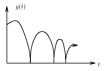
The picture on the left shows the basic properties of a bouncing ball which is thrown into a box from the upper left. The bouncing height of the ball is slowly increasing due to air friction since it is assumed that the interaction of the ball and the bottom is completely elastic so no energy is dissipated there. |
|
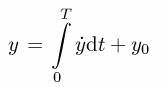
To determine the y position of the ball it is sufficient to integrate over the ball's velocity with respect to time as shown on the right. The dot over y denotes its first derivative with respect to time while y0 is the initial position of the ball. |
|
|
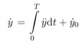
Where does the ball's velocity come from? Obviously from another integration operation which works on the ball's acceleration as shown on the left. The two dots over y denote the second derivative with respect to time while y-dot-0 is the initial accleration of the ball (which might have been thrown to the bottom). |
|
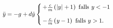
The question remains where this acceleration value comes from. Its equation is shown on the right and consists of two parts in general. The upper part holds when the current position of the ball is below the bottom where it rebounces (since the ball is made from elastic material it will be compressed and excert a force which will drive it back again. The lower part holds if the ball should bounce into the ceiling of the box where it bounces. To keep the simulation simple this effect will not be implemented so the lower part of the equation simplifies accordingly. -g is the acceleration due to gravitation, +d y-dot is the damping due to air friction which is assumed to be proportional to the ball's velocity. Since we assume that there is no ceiling existing that can be hit by the ball, the lower part of the equation is just this - a ball in free fall and slowed down by air friction. When the ball hits the bottom an additional term has to be taken into acount - the force excerted by the deformed ball which tends to get back into its original shape (elastic rebounce, not plastic). |
|
|
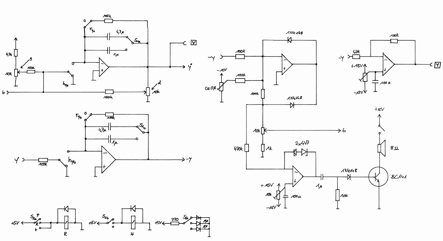
To solve this differential equation of second degree two electronic integrators and a summer are necessary. Since every active component like an integrator and summer will change the sign of its result once we will either get the ball's position or velocity with inverse sign, so an additional summer will be necessary to change the sign again. To control the loudspeaker the acceleration excerted by the compression of the ball hitting the bottom has to be shaped accordingly and amplified which takes yet another operational amplifier as well as a transistor to drive the loudspeaker. All in all the simulator needs five operational amplifiers, one NPN transistor and two relays for the necessary integrator control. The circuit of the simulator is shown in the picture below. Please note that the power supply I built is way too complex - this was the result of me a) not thinking far enough and b) thinking about a more complex simulation circuit which would have taken the x-position of the ball into account, too. Thus the schematics shown are a bit simplified and only need +/- 15 V as well as a +5 V supply, so be not puzzled if the schematic does not match my breadboard implementation shown below. The circuit itself is rather simple and straight forward - both integrators use to double throw relay switches for control of the the three possible operating modes (initial condition, compute, halt) while the first mode, initial condition, is rather simple since zero is the default initial condition for both integrators so only the capacitors have to be discharged. Click on the schematic picture below to get a high resolution JPG image or click here to get the schematic as PDF file. Switch 1 is used to select beween fast and slow running mode by selecting one of two possible feedback capacitors of the two integrators. Switch 2 is used to select between the three modes of operation (initial condition, run, halt).
|
|
|
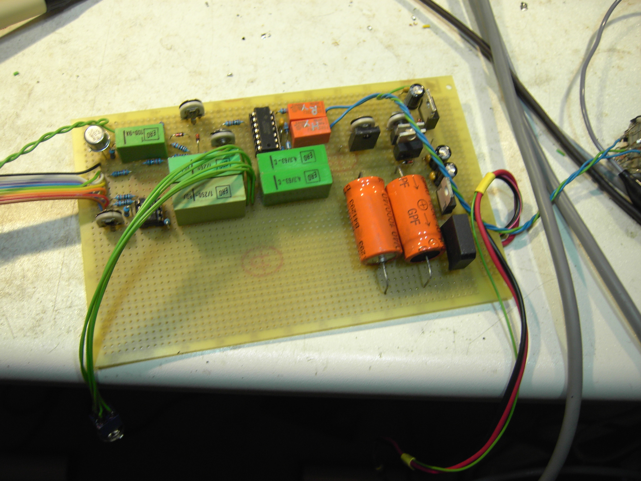
The picture on the left shows the parts side of the bouncing ball simulator. On the right is the (way too complicated :-) ) power supply which generated +/- 15 V, +/- 10 V and +5 V. Next to it on the left is the quad operational amplifier TL084 with its associated two orange relays for the control of the two integrators. Three of its amplifiers are actually needed for the ball simulation. The fourth amplifier is a comparator for generating the bouncing sound. |
|
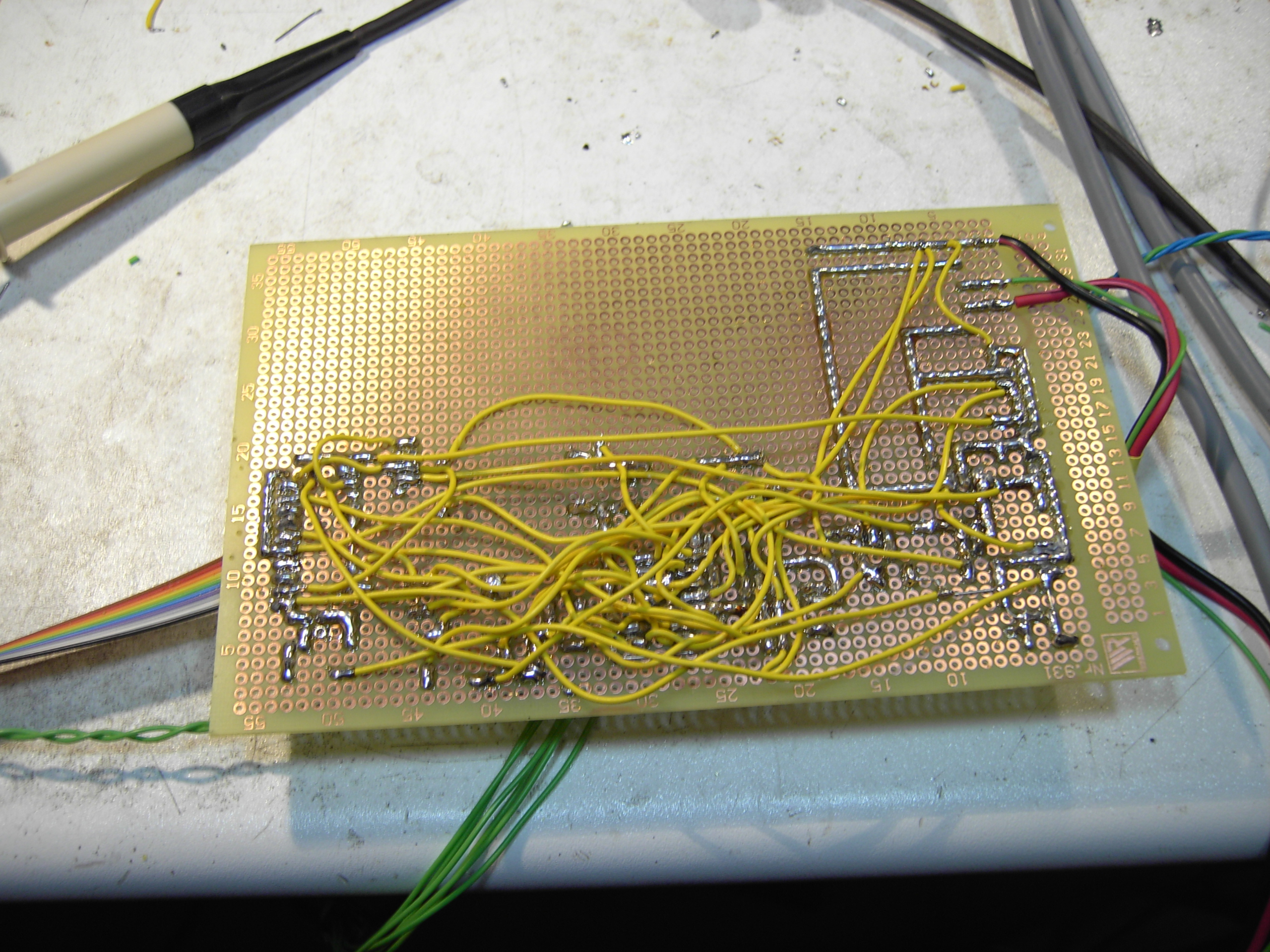
The picture on the right shows the rather crowded soldering side. The reason why the board is so densly populated is that I initially planned to generate a X-deflection generator, too, but abandoned that idea due to the lack of time. |
|
|
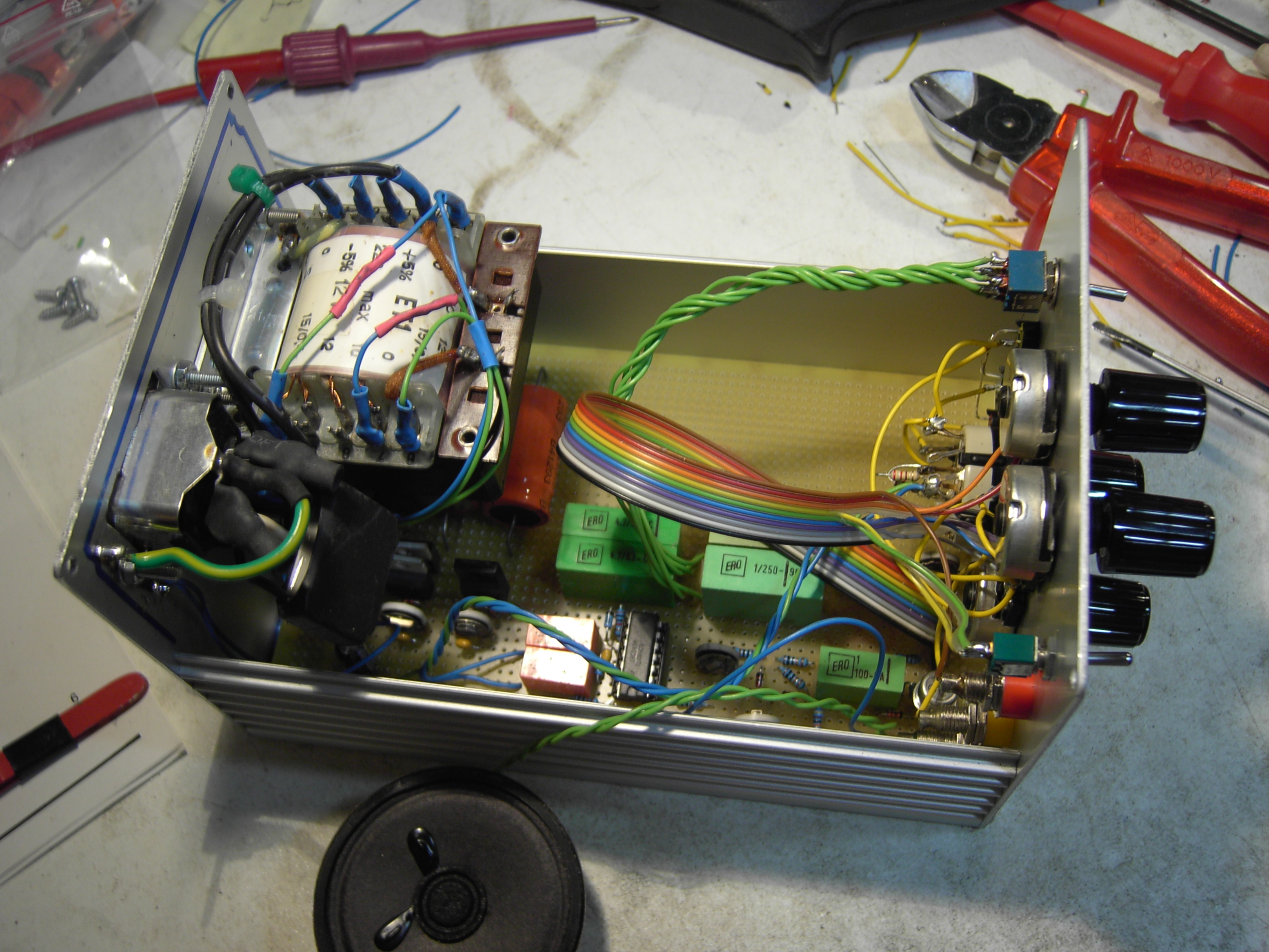
The picture on the left shows the overall device with its power supply transformer on the left hand side and the control panel on the right. On the bottom of the picture the currently unmounted loudspeaker can be spotted. |
|
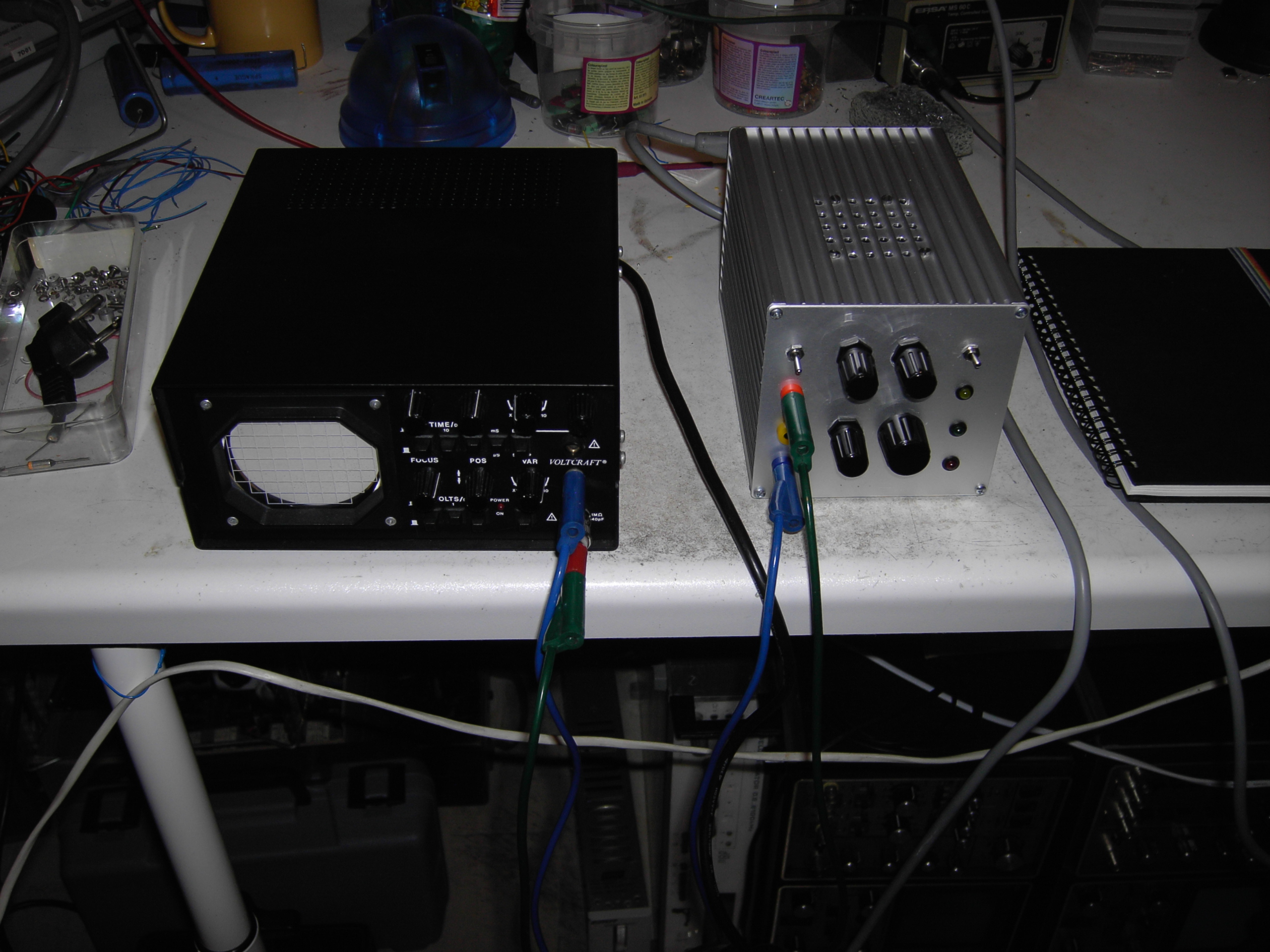
The overall system setup can be seen in the picture on the right. On the left is a very basic Voltcraft oscilloscope which is perfect for travelling and showing a live demo while the bouncinc ball simulator box can be seen on the right. There are three potentiometers on its control panel: Damping, gravitation and elasticity of the ball. The big switch on the lower right is used to select the desired mode of operation (initial condition, compute, halt). The two small switches on the top are for the loudspeaker and the overall simulation speed (fast / slow). |
|
|
Here you can find a short (1.5 MB) AVI-video showing the performance of the bouncing ball simulator. The same video may be downloaded from youtube here. |
|
|
26-APR-2009, 10-MAY-2009, ulmann@analogmuseum.org |
|