Two-dimensional simulation of a spaceship

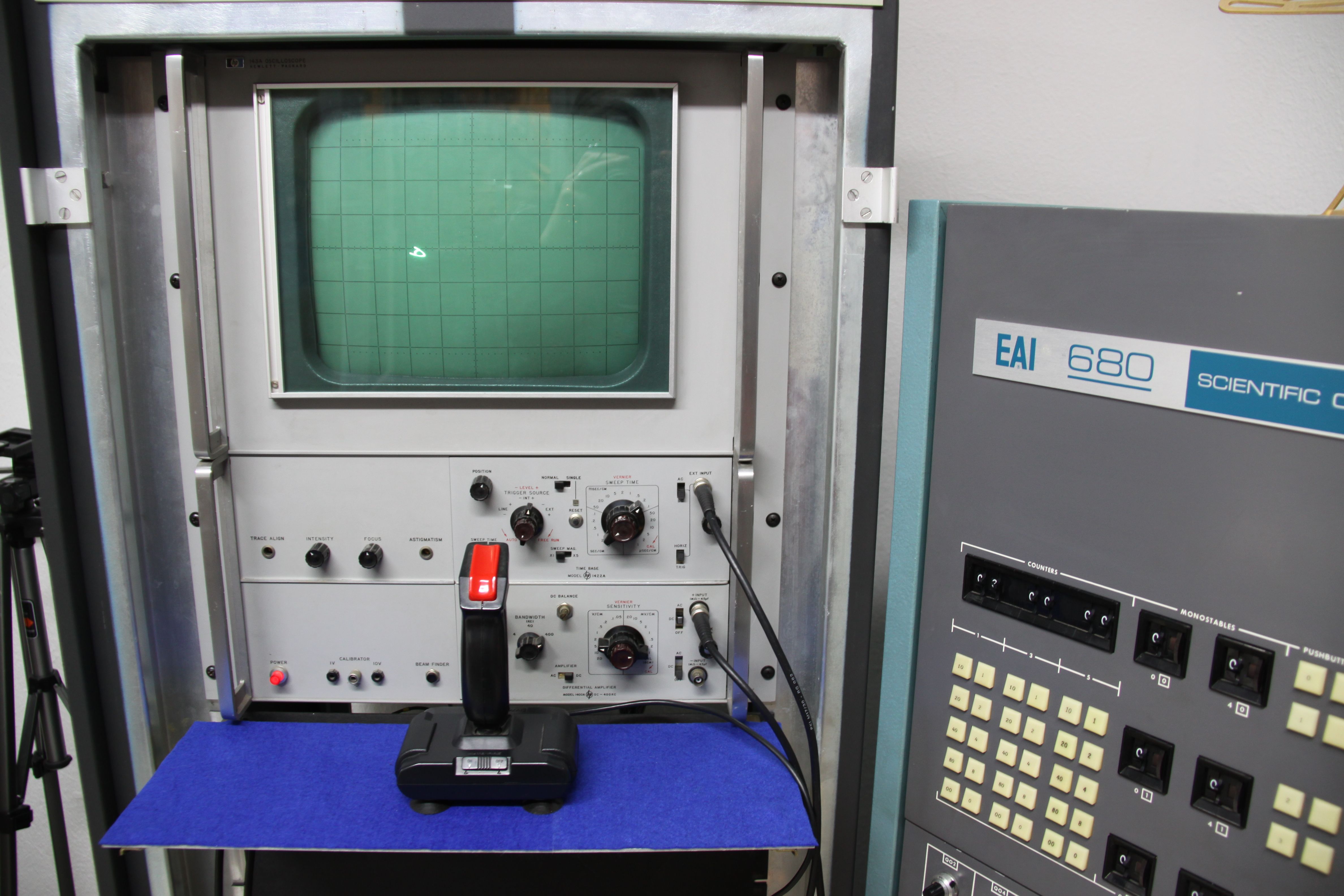
Now (May 2014) that my EAI 680 is more or less working, I couldn't wait to setup a somewhat more complex simulation. As I am an avid reader of NASA reports from the Mercury, Gemini, and Apollo era, the idea of implementing a simple two-dimensional simulation of a spacecraft came to my mind. The picture above shows the the setup of the finished program. The spacecraft is displayed on a large screen oscilloscope. In front of this display a simple Quickshot II joystick is mounted which is used to control the thrusters of the spaceship.

The simulated spaceship has two sets of thrusters which can be controlled by the joystick: Two thrusters are located on the front and back of the spacecraft and allow positive/negative thrust along its longitudinal axis. The second set of thrusters is mounted in a way that the spaceship can be rotated.

As there is no friction, the rotational and translational movements of the spaceship do not slow down (which feels extremely awkward for someone like me who is not used to play computer games :-) ). The thrusters have only two states: Quiescent and operating. They are not throttleable.

The circuit is not too complicated but requires a lot of multipliers to implement the rotation matrix as will be shown in the following detailed circuit description.

First of all, the shape of a spacecraft has to be generated for the display. The typical approach is to generate a sine/cosine-signal pair and distort one component by means of a diode function generator in a suitable way to generate the overall appearance of a spaceship. Generating such a sine/cosine-signal pair is simple and is based on the following differential equation: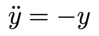

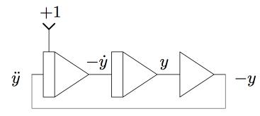
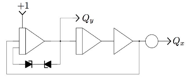
This differential equation can be easily solved by the basic computer setup shown on the right. Assuming that the second derivative of the function is known, its first derivative (with reversed sign due to the implementation of the integrators) can be obtained by means of an integrator. A second integrator yields y, and an inverter (i.e. a summer with only input) yields -y. Since -y is equal to the second derivative of y by definition (see above), we can now setup a feedback path in this simple computer circuit by feeding -y into the input of the integrator chain. The leftmost integrator is also fed with +1 as its initial condition to avoid the trivial zero solution of the above differential equation.

Since analog computer elements are not perfect, the amplitude of the output signals generated by this basic circuit will not be constant. In the case of my EAI 680 the integrators exhibit a small positive error so that the amplitude will not decay but will eventually overload the circuit. Therefore an amplitude limiter (two Zener-diodes in series connected between the output of the first integrator and its summing junction) has to be provided as shown below:

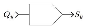
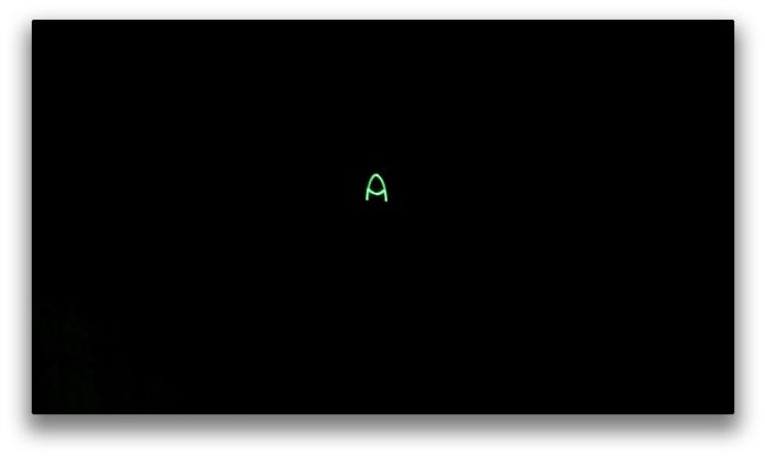
Both integrators have to be setup with a short time constant thus yielding a rather high-frequency sine/cosine-signal pair (several kHz are easily achieved). If the two outputs of this circuit are connected to the X- and Y-inputs of an oscilloscope, a circle will be displayed.

Using a diode function generator (suitably set up), shown on the right, the y-component generated by this sine/cosine-circuit can be distorted in a way that the outline of a (simple :-) ) spacecraft will be displayed on the oscilloscope.

Now that we can display the figure of a spacecraft on an oscilloscope, we have to deal with the control joystick. The circuit shown below generates an angular rate output controlled by the left/right movement of the joystick. The two switches of the joystick control the position of a comparator switch as well as the mode of operation of the integrator shown on the right. As long as no switch is activated, the integrator will be in HOLD mode. When one of the two switches closes, the integrator will go into OPERATE mode and integrate over the thrust generated by the rotational thrusters as determined by the potentiometer connected to the output of the comparator switch, thus yielding an angular velocity signal phi-dot.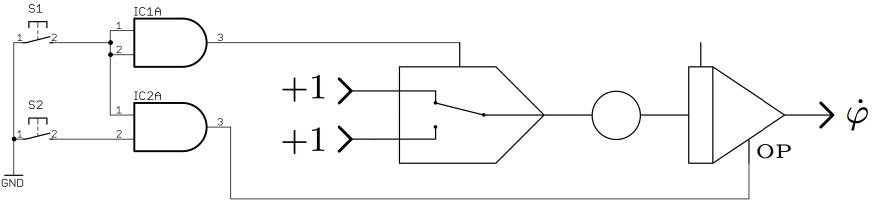

The circuit for the translational thrusters is quite similar but two comparator switches are necessary since the double integration over the thrust signal will be performed later as the thrust must be split into two vector components along the X- and Y-axis of the reference coordinate system.

Now that we have the angular velocity of the spacecraft as generated be the circuit shown above yielding phi-dot, we have to generate a sine/cosine-signal pair depending on phi. A straightforward approach could be based on integrating over the angular velocity to get the angular position phi and feed this signal into a sine- and a cosine-function generator. Unfortunately, this would cause problems as soon as the spacecraft has completed one revolution and starts the next since the value of the angular position would exceed its maximum (or minimum) value, thus overloading the associated computing elements. A much more elegant solution of this problem is based on the simple differential equation y''=-y as shown at the very beginning of this page. Using two multipliers in series, the frequency of the sine/cosine-signal pair generated by the basic setup for this equation can be determined, thus yielding a function generator circuit generating sin(phi) and cos(phi) from phi-dot. This circuit is shown below: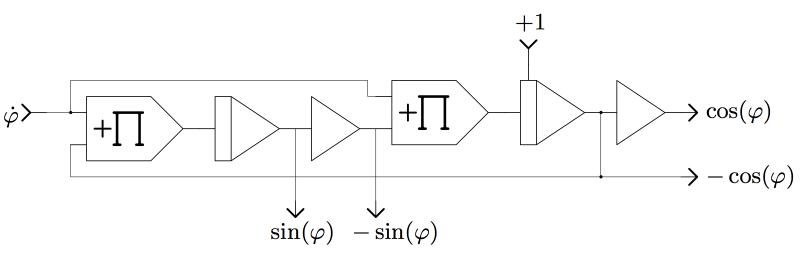

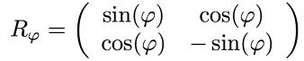
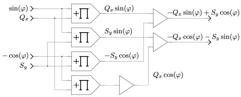
Now that we have sin(phi) and cos(phi), the spacecraft can be rotated by multiplying the vector consisting of its X- and Y-components with the rotation matrix shown on the left. (The unusual signs used here are caused by the repeated sign-reversals caused by the analog computer components.)

Implementing a matrix-vector-multiplication like this is straightforward but requires a lot of multipliers (multiplication is a rather complicated operation for an analog computer, so many analog computers feature only a few multipliers, at best). The circuit performing the actual rotation is shown below:

Now that the spacecraft can be rotated by controlling its rotational thrusters by the joystick, we have to implement its translational movement. This requires splitting the thrust along its longitudinal axis into two components as determined by the angular position of the spacecraft. These two acceleration components are then integrated twice yielding the spacecraft coordinates at which the figure is drawn on the oscilloscope's screen. The necessary circuit is shown below: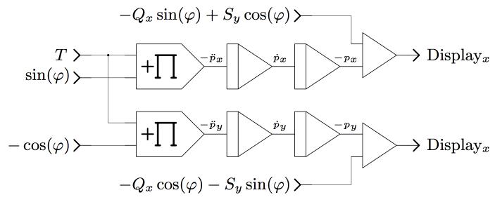

The overall setup of the computer (including me during development of this program) is shown below, followed by a short video demonstrating the simulation (and my poor skills as a pilot :-) ).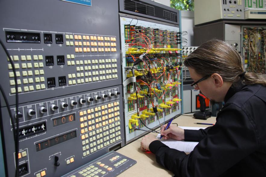

28-MAY-2014, ulmann@analogmuseum.org