| The very first analog computer made by TELEFUNKEN |
| The very first analog computer made by TELEFUNKEN |
|
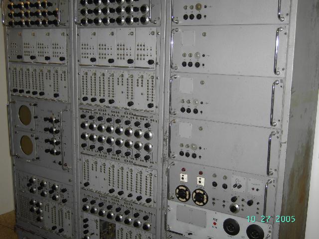
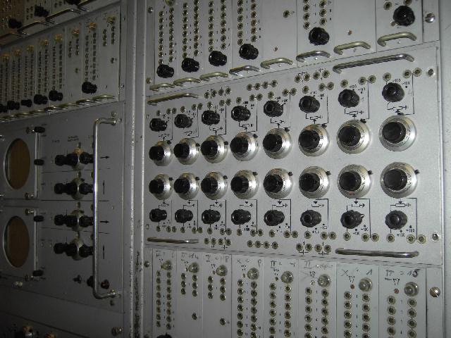
The analog computer shown in the following is the first (analog) computer ever built be TELEFUNKEN. This machine is the engineering model which was developed by Dr. Kettel, Dr. Schmidt, Dr. Kley and others in the time frame from about 1955 to 1956. I was able to identify this system as being the first analog computer made be TELEFUNKEN ever due to personal communication with Dr. Kley who remembered quite vividly some of the exceptional feature of this machine compared with its successor, the production model which was called RA463/2. This machine is based on electron tubes and features a machine unit of +/- 100 V. The system is from the late 1950ies - an exact date of manufacturing is unknown. The picture above shows the overall system - it consists of three 19 inch racks mounted on a pedestal. The right most rack contains the power supplies - from top to bottom these are:
The rack in the middle contains from top to bottom:
The left most rack contains from top to bottom:
Unfortunately the system is not in a good condition - many of its tubes are missing especially those which were accessible from the rear without the need to remove drawers. The system was sitting idle for years in a warehouse which causes the paint to fall down in large pieces, too. The system is incredibly heavy - even for someone devoted to large computer systems like me. Even with all drawers removed the steel frame is so heavy that we had to use a fork lift just to get it on the tail lift of the truck. When we arrived at home we had not only to remove every single drawer but we had to disassemble the steel frame, too, to move the systems nine steps up to the house. Some drawers - especially the power supplies are so heavy that it takes two persons to lift them back into the rack. Wanted: I am desperately looking for documentation about this system. Most wanted are drawings - even from its successor system, the RA463/2. I also need a source for the very special patch cords used by TELEFUNKEN. These are completely incompatible to the cords used in the RA800 or RA770. The following pictures show some of the system's components in greater detail: |
|
|
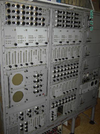
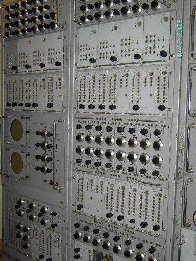
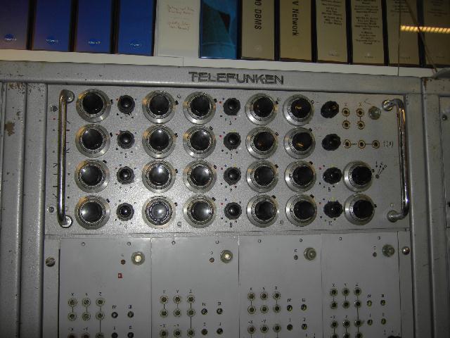
Front: The system is really beautiful as the following pictures show. Quite remarkable in my oppinion is the fact that this machine does not have a central patch panel where all connections of the computing elements are routed to. Instead every drawer has some plugs on its front which are used to interconnect the computing elements during a calculation. This makes it quite difficult to change a program - one has to remove all patch cords which run over the entire front of the computer in order to make room for the next program. |
|
|
|
|
|
|
Coefficient potentiometers, free diodes and relais: The small drawer on the left contains five coefficient potentiometers of 50 k Ohms each. There is no overload protection for the potentiometers as was usual in later designs. The drawer on the right contains six free diodes (these are implemented using three EAA91 tubes) and four fast relais which are normally controlled by comparators. |
|
|
|
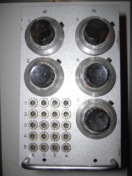
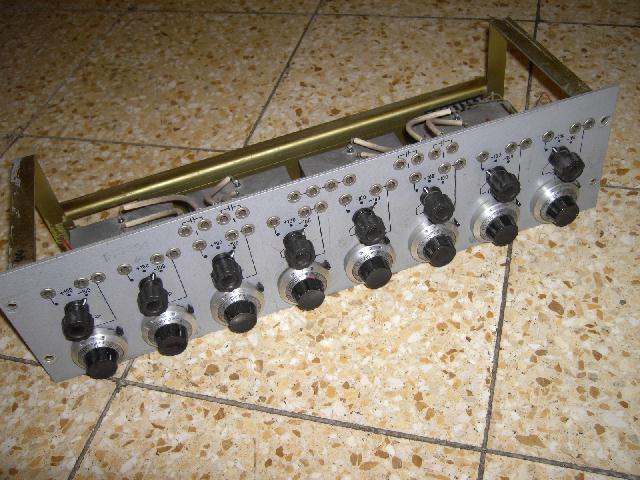
| The drawer on the left contains sixteen coefficient potentiometers which can be used as free potentiometers, as voltage dividers or as initial value potentiometers (in the latter case the potentiometer acts as a voltage divider between ground and + or - 100 V). The picture on the right shows a smaller version of this drawer containing only eight potentiomers. This drawer also contains four free precision capacitors. | |
|
|
|
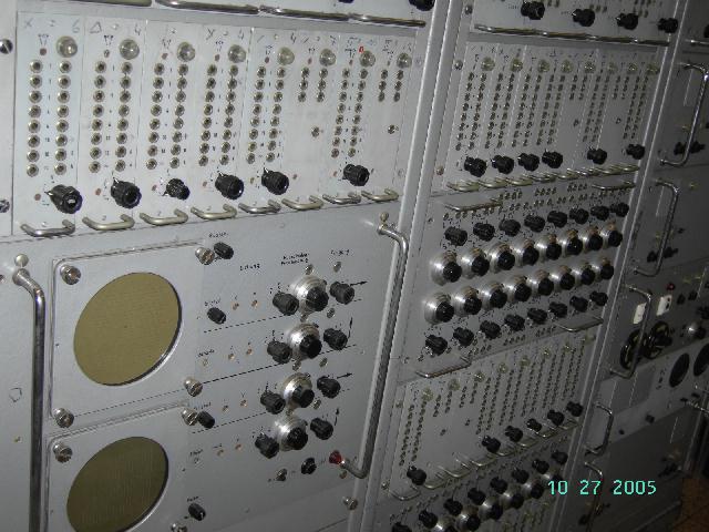
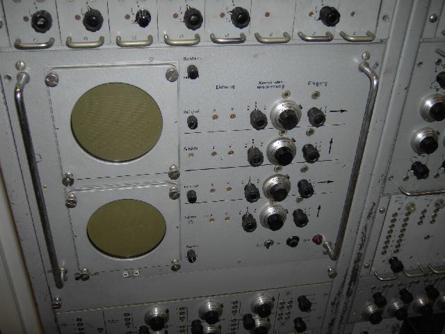
Oscilloscope, function generator, summers/integrators: The oscilloscope of this analog computer is a true marvel - in fact it consists of two independent oscilloscope systems mounted above each other. Both oscilloscopes do not have a time base system since they are run as x/y-displays. If a time proportional x-deflection is necessary this can be easily achieved by connecting the output of the system timer, which is nothing else than a high precision integrator with a comparator, with the x-input of the oscilloscope. |
|
|
|
| The picture on the left below shows one of the two diode based function generators of the computer. The potentiometers are used to control the first derivative of a polygon spanning from -100 V to +100 V at fixed x-intervals. The picture on the right shows one of the drawers containing multiple summers/integrators. These form the heart of every analog computer. | |
|
|
|
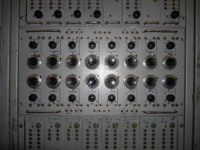
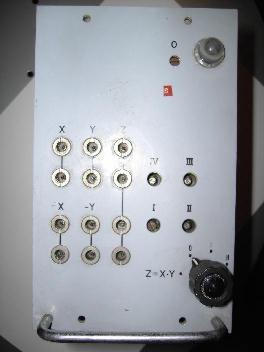
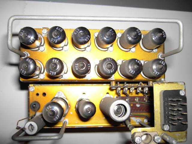
Parabola multipliers: The parabola multipliers of the RA 1 are very interesting devices - as in most small to medium analog computers the RA 1 does not have servo multipliers of time division multipliers. Instead its multipliers are based on parabola function generators. The idea behind this is based on the fact that xy = ((x + y)^2 - (x - y)^2) / 4 (try it yourself). So to calculate xy which is quite difficult for an analog computer, the multiplier just calculates two parabola - one for the argument x + y and one for x - y. So only two parabolas have to be calculated which can be done using two diode based function generators which implement a polygon based approximation to a true parabola. The two results from these function generators are then added and divided by 4 (by a simple voltage divider) yielding the output of the multiplier. The picture on the left below shows the front panel of the multiplier unit. The necessity of have +x, -x, +y and -y as input values is a result from the parabola function generator employed. The picture on the right shows the 24 diodes implemented by 12 EAA91 tubes which comprise the two parabola function generators, so each parabola is approximated by a polygon of 12 sections. |
|
|
|
|
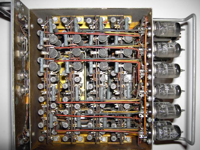
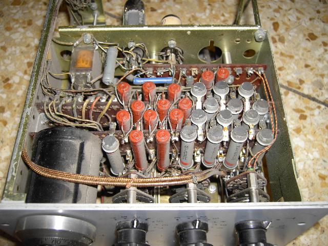
Below left the resistor networks of the two parabola function generators of the multiplier can be seen. These use precision resistors trimmed to the necessary values to approximate the parabola with minimal error. The picture on the right shows the other side of the multiplier drawer which contains the summer for adding the two parabola values and its associated resistor networks. |
|
|

|
|
The system timer: The overall control of a calculation is the task of the system timer. The only non-time invariant computing networks are the integrators so these must be supplied with proper control values. An integrator is in one out of three states at every moment:
|
|
|
|
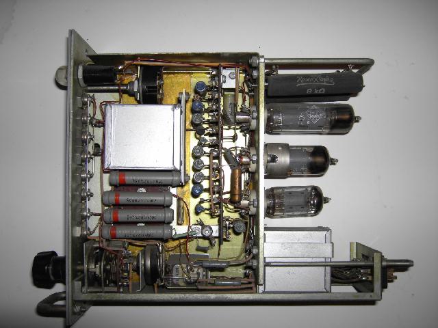
| The two pictures below show the internals of the system timer. Prominent in the left picture is the large integrating capacitor - on the far left a small relais can be seen. The picture on the right shows the precision resistor networks which implement the various time constants. | |
|
|
|
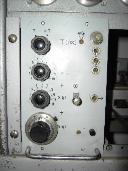
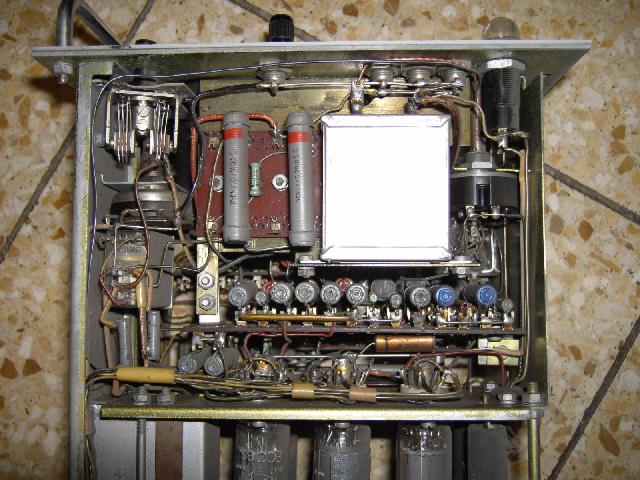
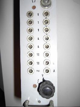
Summer/Integrator: The pictures below show one of the summers/integrators which are the heart of the system. Each of these amplifiers can be changed from acting as a summer to an integrator by setting the switch at the bottom. The inputs of the summer/integrator are weighted with weights of 1, 4 and 10 respectively. The input marked with the infinity sign is the summing point of the amplifier and can be used to setup additional feedback paths (like free diodes for limiters/comparators, etc.). |
|
|
|
| 17-DEC-2005, 04-MAY-2006, 26-JAN-2008 |